Boston House Price Predictor
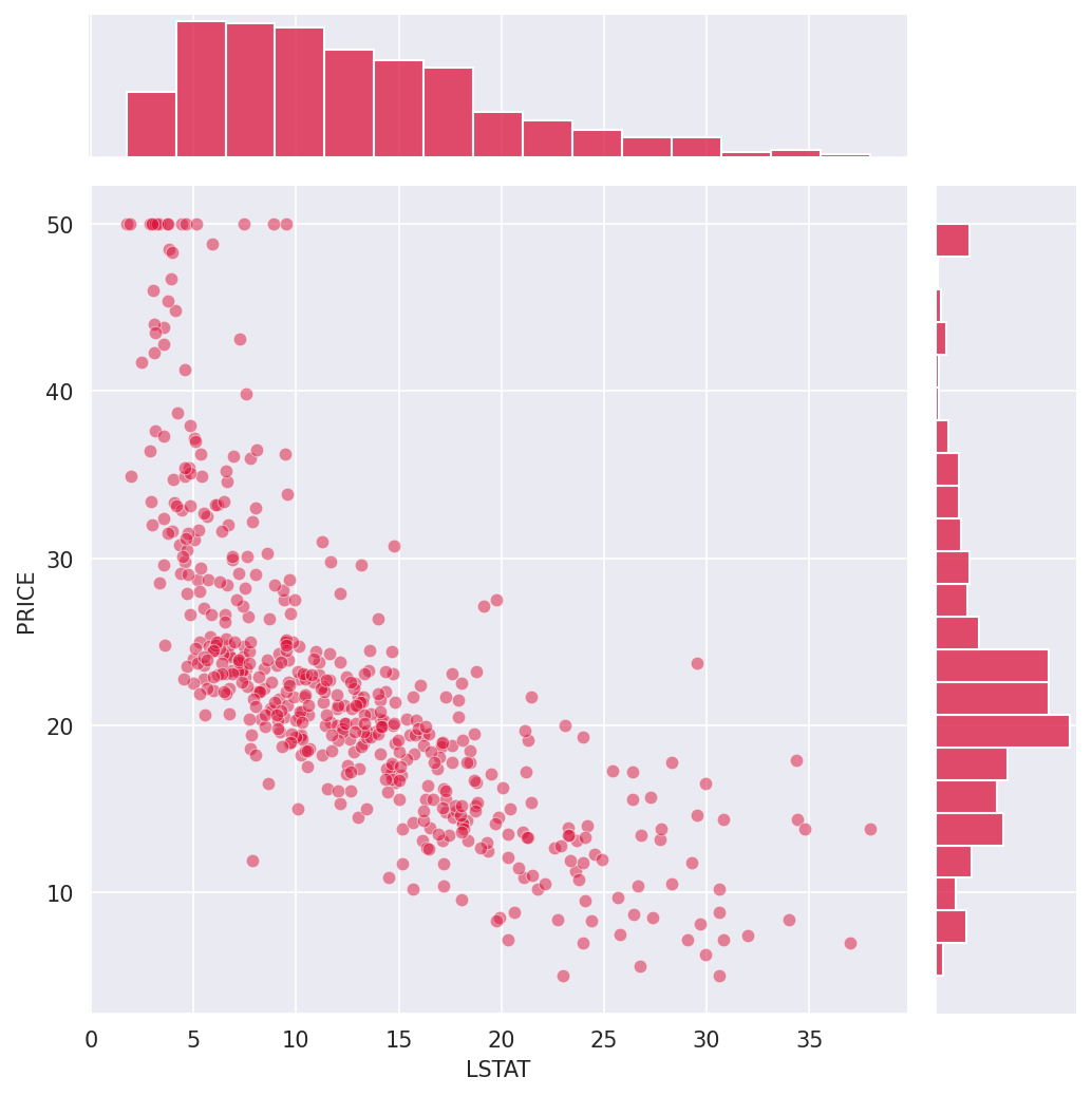
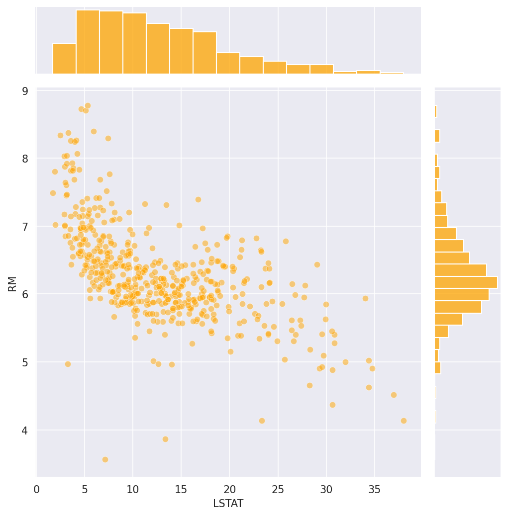
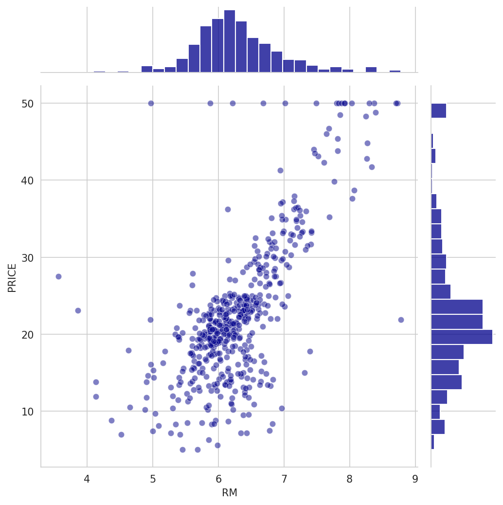
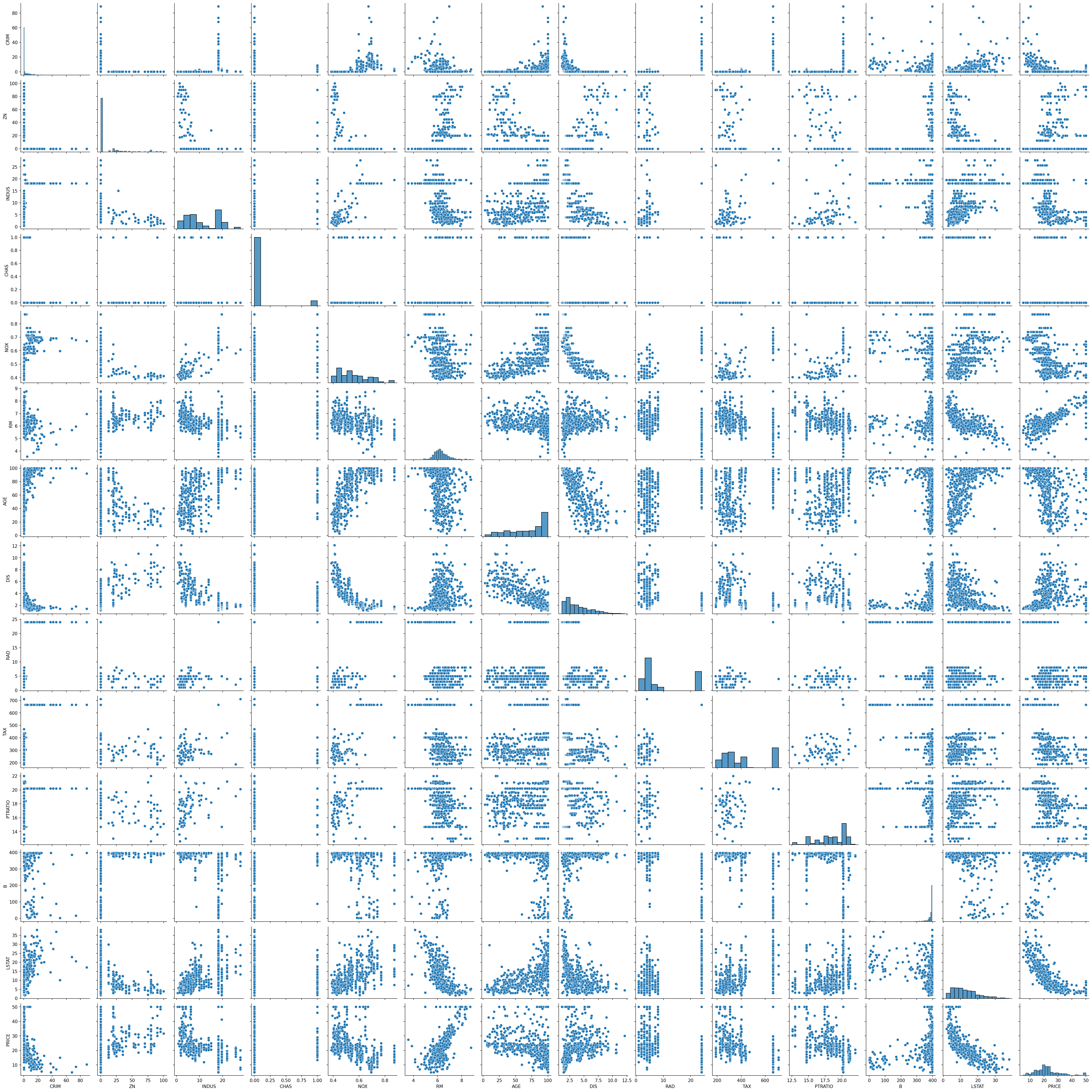
This project works through 506 Boston census tracts from the Harrison & Rubinfeld (1978) dataset, fitting a multivariable linear regression across 13 socio-economic and geographic features to explain median residential property values. The pipeline covers data cleaning, exploratory visualisation (distributions, pair plots, joint plots), an 80/20 train/test split, residual diagnostics, and a working valuation function.
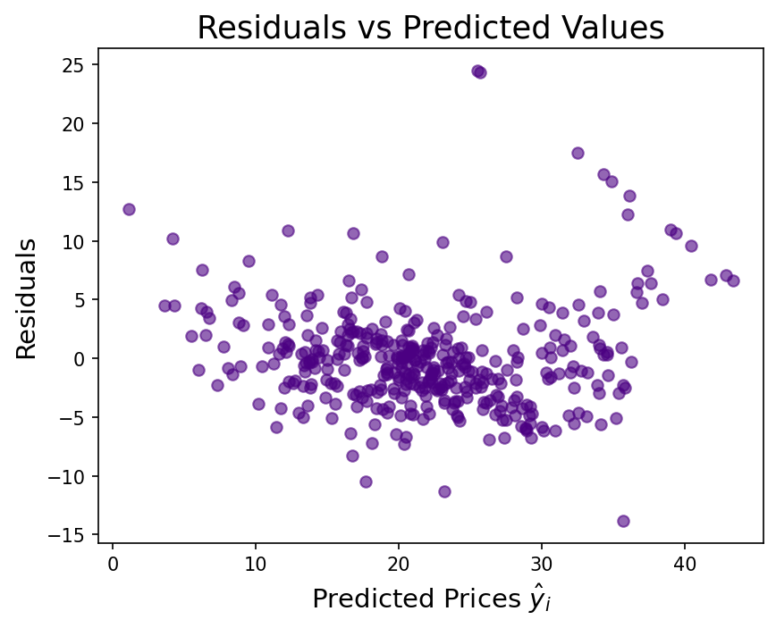
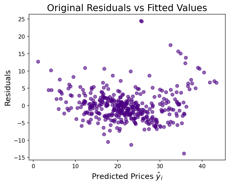
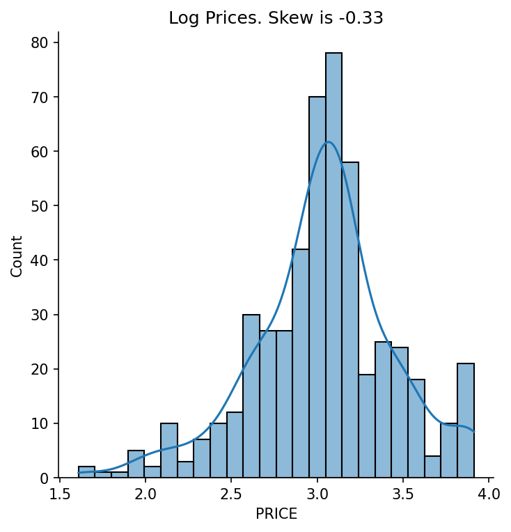
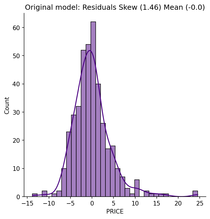
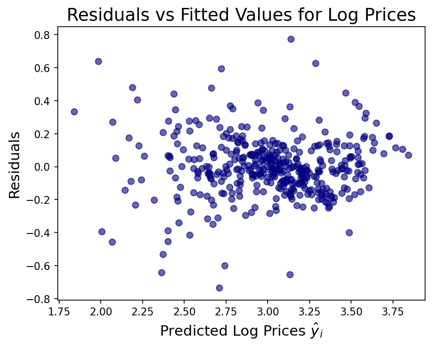
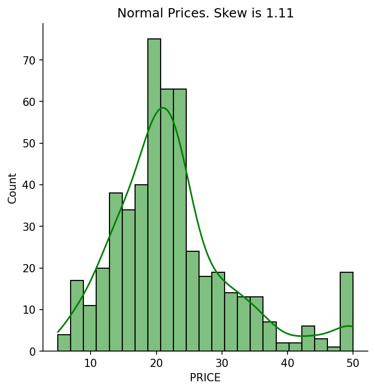
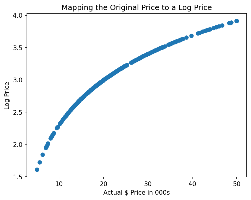
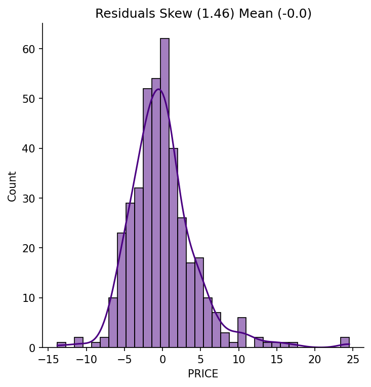
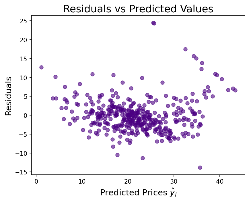
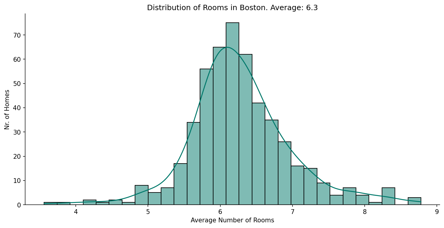
The raw price distribution carries a positive skew (1.46) that inflates the residuals. Applying a log transformation to the target reduces residual skew to 0.09 and lifts test-set r² from 0.67 to 0.74. Number of rooms is the strongest positive predictor (each additional room adds ~$3,109). Nitric oxide pollution carries the largest negative coefficient (−0.70). River proximity raises estimated prices; poverty level and pupil-to-teacher ratio both depress them.
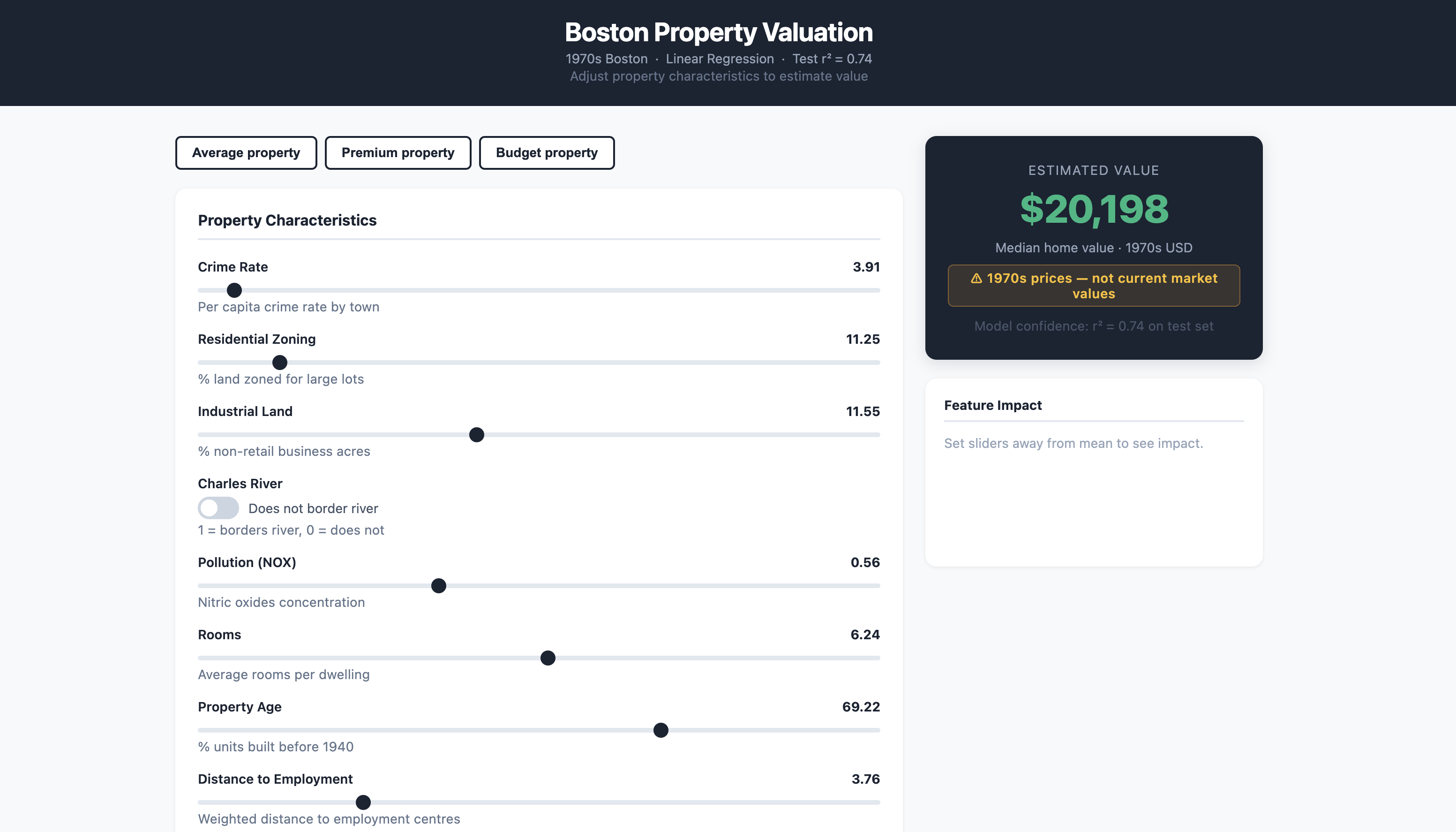
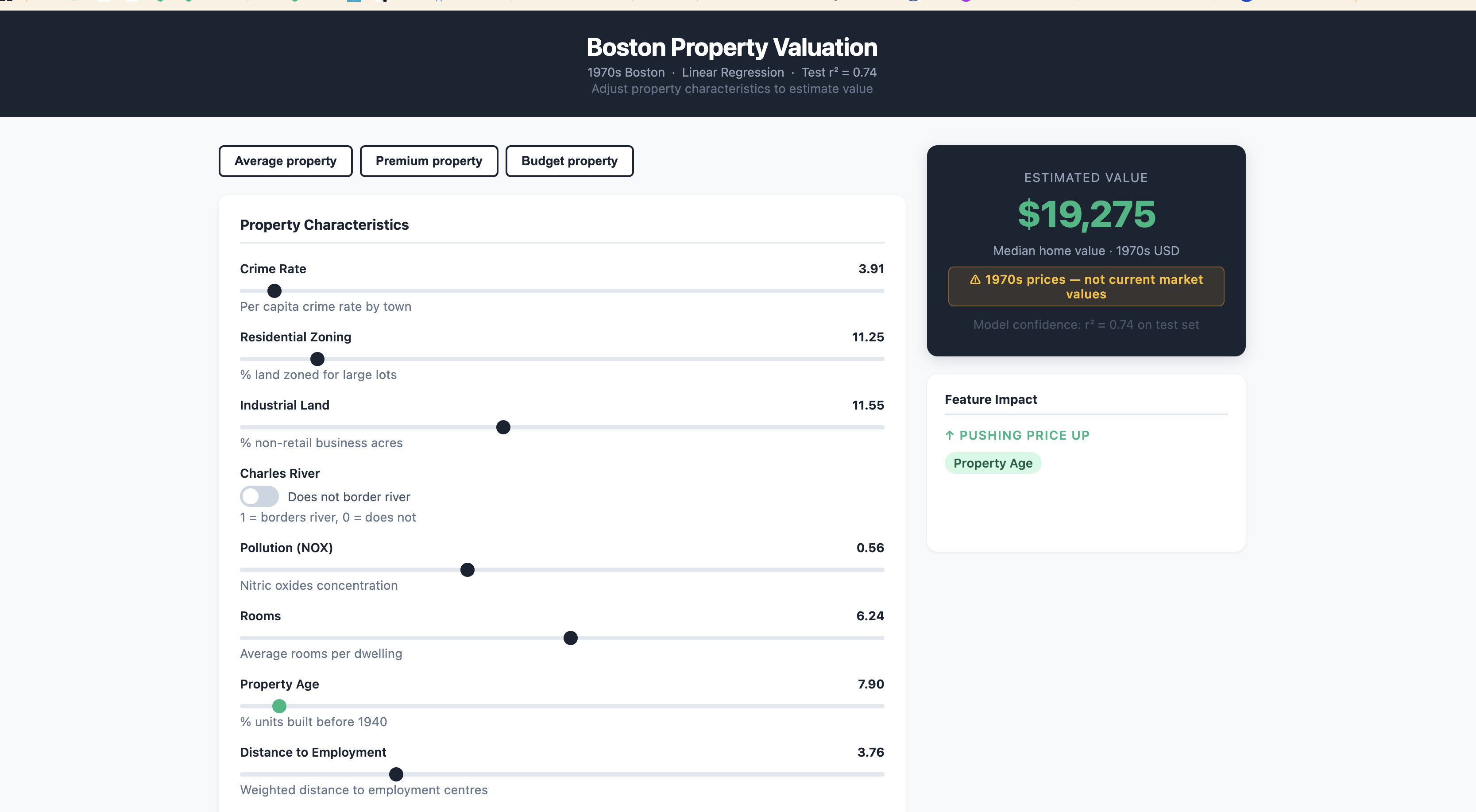
The deployed app exposes all 13 features as interactive sliders. Adjusting rooms, pollution, crime rate, or river proximity updates the estimated property value in real time. A feature impact panel shows which characteristics are currently pushing the price up or down — making the model's internal logic visible without showing raw coefficients.
Key results: average Boston property estimated at ~$20,198; an 8-room river-front property in a low-poverty area estimates at ~$37,110. All prices are 1970s USD.
Quick Facts
Overview
Problem
Real estate valuation depends on dozens of overlapping factors — proximity to employment, school quality, crime, pollution, room count — and it is not obvious which factors matter most or by how much. The goal was to quantify these relationships for 1970s Boston and deploy the model as a live interactive tool rather than leaving it static in a notebook.
Solution
A multivariable OLS regression fitted on 13 features after an 80/20 train/test split (random_state=10). Log transformation applied to the target after residual diagnostics confirmed skew. Coefficients interpreted for sign and magnitude; np.exp() inverts the log transform at inference time. FastAPI wraps the trained model (StandardScaler + LinearRegression stored as joblib pkl files) and serves a single-page slider UI. Deployed to Azure App Service (F1 free tier) via zip deploy.
Challenges
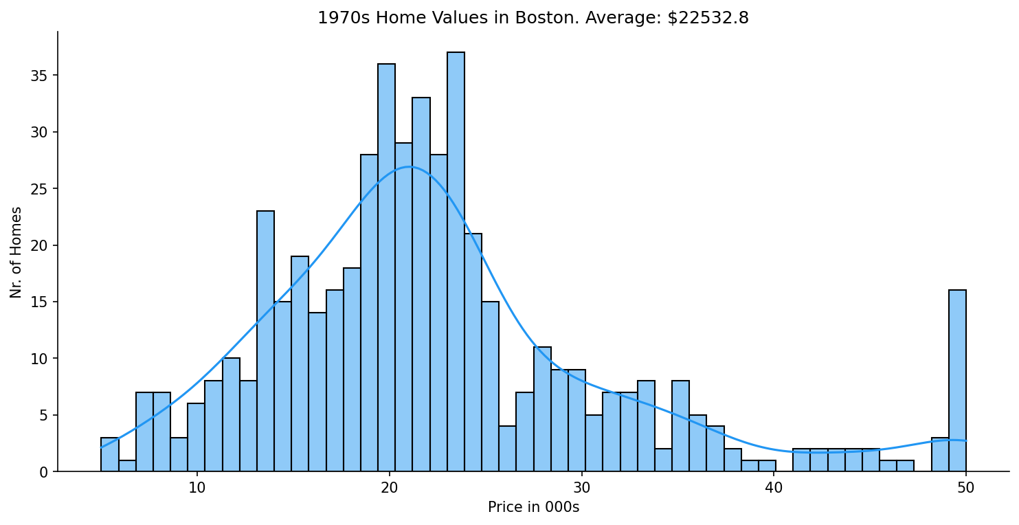
The raw price distribution has a pronounced right skew (1.46), driven partly by a hard cap at $50,000. Validating that the log transformation genuinely helped — rather than just appearing to — required comparing residual distributions and both train and test r² across both models. The improvement in test r² (0.67 → 0.74) and residual skew (1.46 → 0.09) confirmed it was warranted. On the deployment side, the log transform must be reversed at inference (np.exp(prediction) × 1000) and the existing notebook CI workflow had to be preserved alongside the new API test workflow without conflict.
Results / Metrics
- Log model test r²: 0.74 (vs. 0.67 raw)
- Log model train r²: 0.79 (vs. 0.75 raw)
- Residual skew reduced from 1.46 to 0.09
- Each additional room adds ~$3,109 to estimated value
- Pollution (NOX) is the strongest negative predictor (coefficient −0.70)
- Average Boston property: ~$20,198 · Premium 8-room river-front property: ~$37,110
- All prices are 1970s USD — not current market values
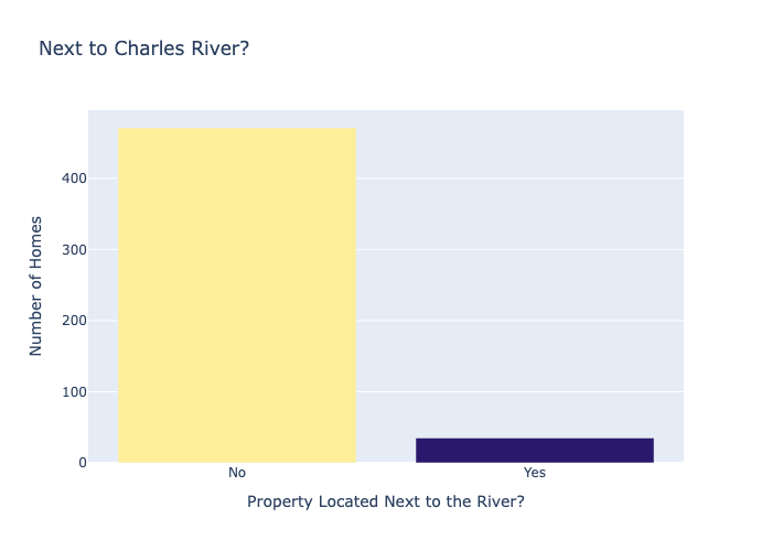
- 35 of 506 properties border the Charles River
Screenshots
Click to enlarge.
Click to enlarge.